Competition Among Servers in Attracting Newcomers

How does mastodon.social factor into the aggregate Mastodon onboarding process?

: The main page of mastodon.social as viewed by a logged out web browser on November 1, 2020. The sign-up form is blurred out and instead there is a message suggesting to either sign up on mastodon.online or see a list of servers accepting new accounts at joinmastodon.org.

Throughout its history, Mastodon’s flagship server, mastodon.social, has allowed and disallowed open sign-ups at various times. When the website did not allow sign-ups, it displayed a message redirecting those interested in signing up for an account to mastodon.social or alternatively to a list of potential servers at joinmastodon.com.

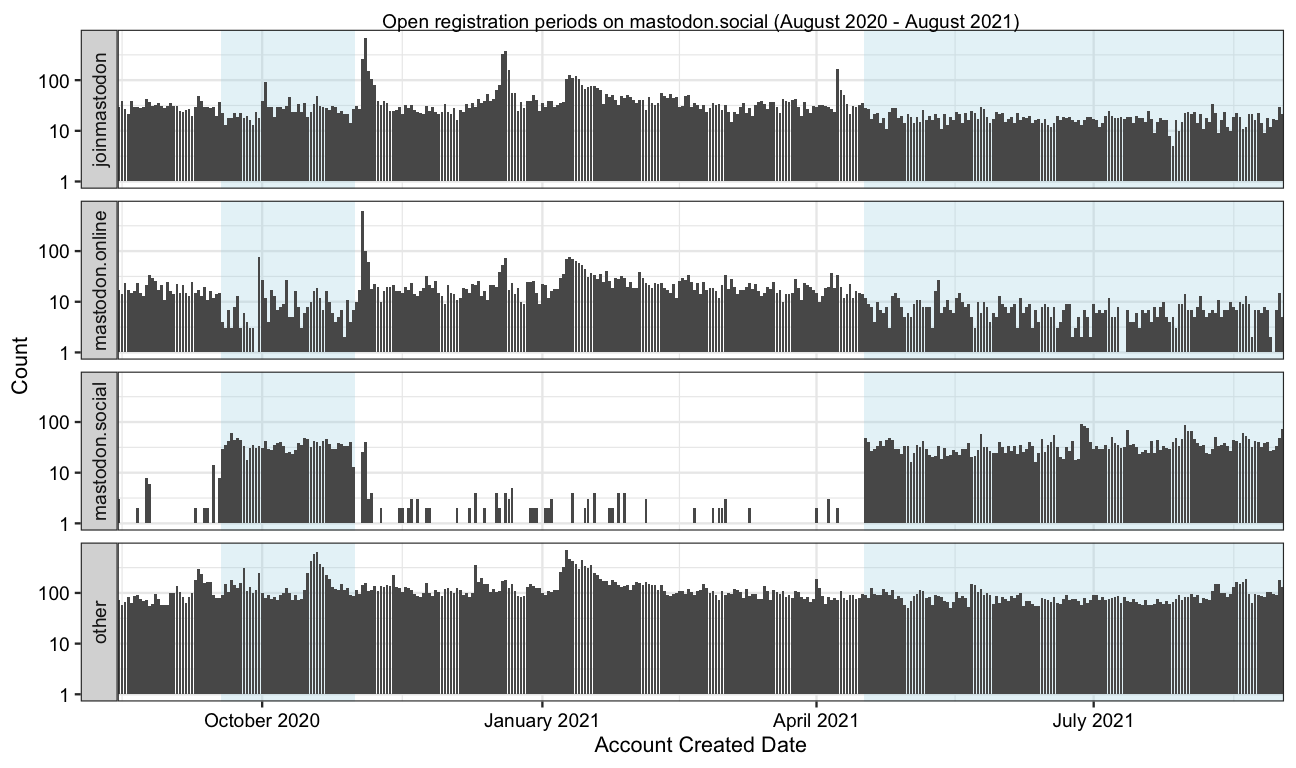
We found three main periods during which mastodon.social did not accept new signups by first noting the times where the proportion of new accounts on mastodon.social drops to zero. We then used the Internet Archive to verify that signups were disabled during these periods.

An extended period of through the end of October 2020.
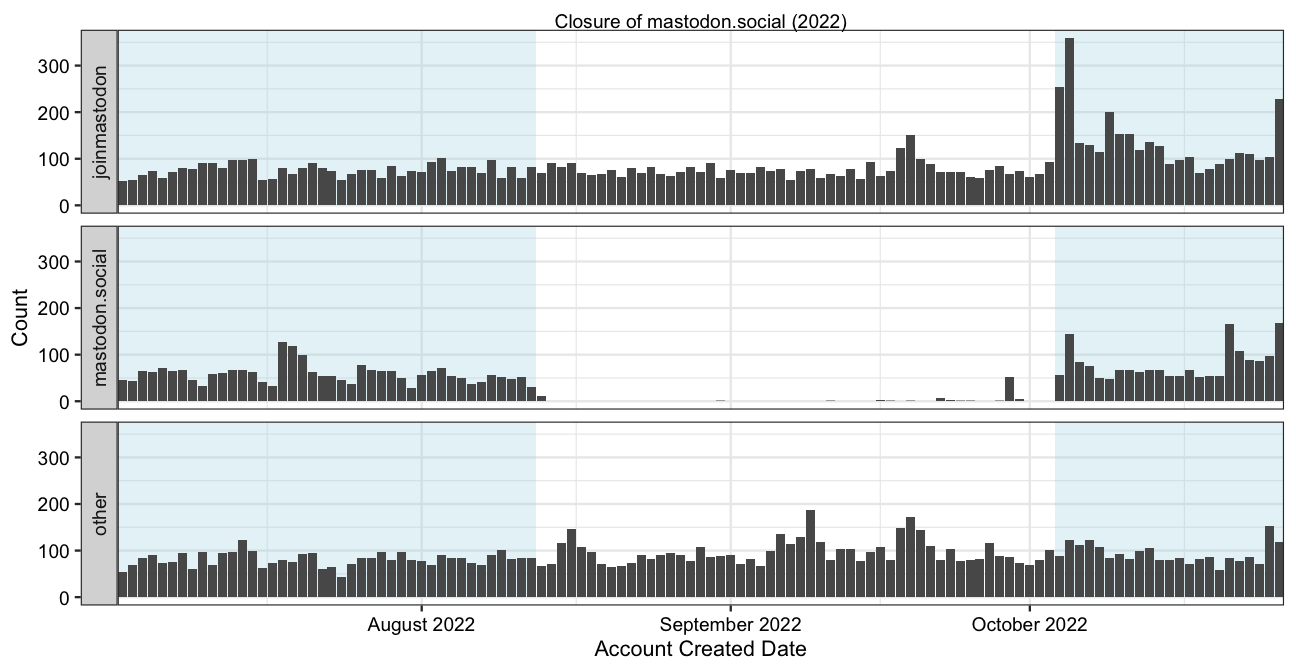
A temporary issue when the email host limited the server in mid-2022.
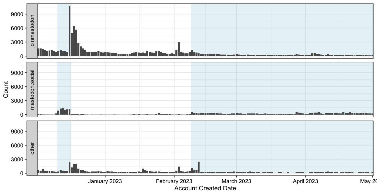
Two periods in late 2022 and early 2023.

We construct an interrupted time series using an autoregressive integrated moving average (ARIMA) model for sign-ups on mastodon.social, the servers linked in joinmastodon.org, and all other servers. For the first period, we also include mastodon.online since mastodon.social linked to it directly during that time.

\[ \begin{aligned} y_t &= \beta_0 + \beta_1 \text{open}_t + \beta_2 \text{day}_t + \beta_3 (\text{open} \times \text{day})_t \\ &\quad + \beta_4 \sin\left(\frac{2\pi t}{7}\right) + \beta_5 \cos\left(\frac{2\pi t}{7}\right) \\ &\quad + \beta_6 \sin\left(\frac{4\pi t}{7}\right) + \beta_7 \cos\left(\frac{4\pi t}{7}\right) \\ &\quad + \phi_1 y_{t-1} + \phi_2 y_{t-2} + \epsilon_t \end{aligned} \]

where \(y_t\) is the number of new accounts on a server at time \(t\), \(\text{open}_t\) is a binary variable indicating if the server is open to new sign-ups, \(\text{day}_t\) is an increasing integer represnting the date, and \(\epsilon_t\) is a white noise error term. We use the sine and cosine terms to account for weekly seasonality.

Results from ARIMA models for the number of new accounts on mastodon.social, mastodon.online, servers linked in joinmastodon.org, and all other servers.
Period	Setting	Significant
2020-2021	mastodon.online	Yes
	JoinMastodon	No
	Other	No
Mid 2022	JoinMastodon	No
	Other	No
Early 2022	JoinMastodon	No
	Other	No

Appendix

Push and Pull Model

In [1]:

#| echo: false
#| output: false
#| warning: false
#| label: push-pull-prep
library(arrow)


Attaching package: 'arrow'

The following object is masked from 'package:utils':

    timestamp

#| echo: false
#| output: false
#| warning: false
#| label: push-pull-prep
library(tidyverse)

── Attaching core tidyverse packages ──────────────────────── tidyverse 2.0.0 ──
✔ dplyr     1.1.4     ✔ readr     2.1.5
✔ forcats   1.0.0     ✔ stringr   1.5.1
✔ ggplot2   3.4.4     ✔ tibble    3.2.1
✔ lubridate 1.9.3     ✔ tidyr     1.3.1
✔ purrr     1.0.2

── Conflicts ────────────────────────────────────────── tidyverse_conflicts() ──
✖ lubridate::duration() masks arrow::duration()
✖ dplyr::filter()       masks stats::filter()
✖ dplyr::lag()          masks stats::lag()
ℹ Use the conflicted package (<http://conflicted.r-lib.org/>) to force all conflicts to become errors

#| echo: false
#| output: false
#| warning: false
#| label: push-pull-prep
library(tsibble)


Attaching package: 'tsibble'

The following object is masked from 'package:lubridate':

    interval

The following objects are masked from 'package:base':

    intersect, setdiff, union

#| echo: false
#| output: false
#| warning: false
#| label: push-pull-prep
library(fable)

Loading required package: fabletools

#| echo: false
#| output: false
#| warning: false
#| label: push-pull-prep
library(lmtest)

Loading required package: zoo

Attaching package: 'zoo'

The following object is masked from 'package:tsibble':

    index

The following objects are masked from 'package:base':

    as.Date, as.Date.numeric

#| echo: false
#| output: false
#| warning: false
#| label: push-pull-prep
library(jsonlite)


Attaching package: 'jsonlite'

The following object is masked from 'package:purrr':

    flatten

#| echo: false
#| output: false
#| warning: false
#| label: push-pull-prep
library(here)

here() starts at /Users/carlcolglazier/Documents/research/junior-sheer

#| echo: false
#| output: false
#| warning: false
#| label: push-pull-prep
source(here("code/helpers.R"))


Attaching package: 'scales'

The following object is masked from 'package:purrr':

    discard

The following object is masked from 'package:readr':

    col_factor

#| echo: false
#| output: false
#| warning: false
#| label: push-pull-prep
accounts <- load_accounts()
jm <- arrow::read_feather(here("data/scratch/joinmastodon.feather"))

In [2]:

#| label: prep-break-one-raw-counts
server_list <- c(
  "mastodon.social", "mastodon.online"
)

early.jm_servers <- as_tibble(fromJSON(here("data/joinmastodon-2020-09-18.json")))$domain

early.day_counts <- accounts %>%
  filter(created_at < "2021-09-01") %>%
  mutate(created_day = as.Date(floor_date(created_at, unit = "day"))) %>%
  mutate(server_code = ifelse(server %in% early.jm_servers, "joinmastodon", "other")) %>%
  mutate(server_code = ifelse(server == "mastodon.social", "mastodon.social", server_code)) %>%
  mutate(server = ifelse(server == "mastodon.online", "mastodon.online", server_code)) %>%
    group_by(created_day, server) %>%
  summarize(count = n(), .groups = "drop") %>%
  as_tsibble(., key=server, index=created_day) %>%
  fill_gaps(count=0) %>%
  mutate(first_open = ((created_day >= "2020-09-18") & (created_day < "2020-11-01"))) %>%
  #mutate(second_open = ((created_day > "2020-11-02") & (created_day < "2020-11-05"))) %>%
  mutate(third_open = (created_day >= "2021-04-17")) %>%
  mutate(open = (first_open | third_open))

early.data_plot <- early.day_counts %>%
  mutate(created_week = as.Date(floor_date(created_day, unit = "week"))) %>%
  ggplot(aes(x = created_day, y=count)) +
  geom_rect(data = (early.day_counts %>% filter(open)),
            aes(xmin = created_day - 0.5, xmax = created_day + 0.5, ymin = 0, ymax = Inf),
            fill = "lightblue", alpha = 0.3) +  # Adjust color and transparency as needed
  geom_bar(stat="identity") +
  facet_wrap(~ server, ncol=1, strip.position = "left") + #, scales="free_y") +
  scale_x_date(expand = c(0, 0), date_labels = "%B %Y") +
  scale_y_log10() +
  labs(
    title = "Open registration periods on mastodon.social (August 2020 - August 2021)",
    x = "Account Created Date",
    y = "Count"
  ) +
  theme_bw_small_labels()

In [3]:

#| label: table-early-open-coefs

if (knitr::is_latex_output()) {
  format <- "latex"
} else {
  format <- "html"
}

model_data <- early.day_counts %>%
  mutate(count = log1p(count)) %>%
  ungroup %>%
  arrange(created_day) %>%
  mutate(day = row_number())

fit <- model_data %>%
  model(arima = ARIMA(count ~ open + day + open:day + fourier(period=7, K=2) + pdq(2,0,0) + PDQ(0,0,0,period=7)))

early.table <- fit %>% tidy %>%
  mutate(p.value = scales::pvalue(p.value)) %>%
  pivot_wider(names_from=server, values_from = c(estimate, std.error, statistic, p.value)) %>%
  select(-c(.model)) %>%
  select(term,
         estimate_mastodon.online, p.value_mastodon.online,
         estimate_mastodon.social, p.value_mastodon.social,
         estimate_joinmastodon, p.value_joinmastodon,
         estimate_other, p.value_other
         ) %>%
  #select(term, starts_with("estimate"), starts_with("p.value")) #%>%
  knitr::kable(
    .,
    format = format,
    col.names = c("Term", "mastodon.online", "", "mastodon.social", "", "joinmastodon", "", "other", ""),
    digits = 4,
    align = c("l", "r", "r", "r", "r", "r", "r", "r", "r"),
    booktabs = T
  )

In [4]:

#| label: prep-break-two-raw-counts
email.jm_servers <- as_tibble(fromJSON(here("data/joinmastodon-2023-08-25.json")))$domain

email.day_counts <- accounts %>%
  filter(created_at > "2022-07-01") %>%
  filter(created_at < "2022-10-26") %>%
  mutate(created_day = as.Date(floor_date(created_at, unit = "day"))) %>%
  mutate(server_code = ifelse(server %in% email.jm_servers, "joinmastodon", "other")) %>%
  mutate(server = ifelse(server == "mastodon.social", "mastodon.social", server_code)) %>%
  #mutate(server = server_code) %>%
  #filter(server != "other") %>%
  group_by(created_day, server) %>%
  summarize(count = n(), .groups = "drop") %>%
  as_tsibble(., key = server, index = created_day) %>%
  fill_gaps(count = 0) %>%
  mutate(open = ((created_day < "2022-08-13") |
                   (created_day > "2022-10-03")))

email.data_plot <- email.day_counts %>%
  #filter(server != "other") %>%
  mutate(created_week = as.Date(floor_date(created_day, unit = "week"))) %>%
  ggplot(aes(x = created_day, y = count)) +
  geom_rect(
    data = (email.day_counts %>% filter(open)),
    aes(
      xmin = created_day - 0.5,
      xmax = created_day + 0.5,
      ymin = 0,
      ymax = Inf
    ),
    fill = "lightblue",
    alpha = 0.3
  ) +  # Adjust color and transparency as needed
  geom_bar(stat = "identity") +
  facet_wrap( ~ server, ncol = 1, strip.position = "left") + #, scales="free_y") +
  scale_x_date(expand = c(0, 0), date_labels = "%B %Y") +
  labs(
    title = "Closure of mastodon.social (2022)",
    x = "Account Created Date",
    y = "Count"
  ) +
  theme_bw_small_labels()

In [5]:

#| label: email-open-coefs

if (knitr::is_latex_output()) {
  format <- "latex"
} else {
  format <- "html"
}

model_data <- email.day_counts %>%
  mutate(count = log1p(count)) %>%
  ungroup %>%
  arrange(created_day) %>%
  mutate(day = row_number())

fit <- model_data %>%
  model(arima = ARIMA(count ~ open + day + open:day + fourier(period=7, K=2) + pdq(2,0,0) + PDQ(0,0,0,period=7)))

email.table <- fit %>% tidy %>%
  mutate(p.value = scales::pvalue(p.value)) %>%
  pivot_wider(names_from=server, values_from = c(estimate, std.error, statistic, p.value)) %>%
  select(-c(.model)) %>%
  select(term,
         estimate_mastodon.social, p.value_mastodon.social,
         estimate_joinmastodon, p.value_joinmastodon,
         estimate_other, p.value_other
         ) %>%
  knitr::kable(
    .,
    format = format,
    col.names = c("Term", "mastodon.social", "", "joinmastodon", "", "other", ""),
    digits = 4,
    align = c("l", "r", "r", "r", "r", "r", "r"),
    booktabs = T
  )

In [6]:

#| label: prep-break-three-raw-counts
late.jm_servers <- as_tibble(fromJSON(here("data/joinmastodon-2023-08-25.json")))$domain

last.day_counts <- accounts %>%
  filter(created_at > "2022-12-01") %>%
  filter(created_at < "2023-05-01") %>%
  mutate(created_day = as.Date(floor_date(created_at, unit = "day"))) %>%
  mutate(server_code = ifelse(server %in% late.jm_servers, "joinmastodon", "other")) %>%
  mutate(server_code = ifelse(server == "mastodon.social", "mastodon.social", server_code)) %>%
  mutate(server = server_code) %>%
  #filter(server != "other") %>%
  group_by(created_day, server) %>%
  summarize(count = n(), .groups = "drop") %>%
  as_tsibble(., key=server, index=created_day) %>%
  fill_gaps(count=0) %>%
  mutate(open = (created_day > "2023-02-08") | ((created_day > "2022-12-10") & (created_day < "2022-12-17")))

last.data_plot <- last.day_counts %>%
  #filter(server != "other") %>%
  mutate(created_week = as.Date(floor_date(created_day, unit = "week"))) %>%
  ggplot(aes(x = created_day, y=count)) +
  geom_rect(data = (last.day_counts %>% filter(open)),
            aes(xmin = created_day - 0.5, xmax = created_day + 0.5, ymin = 0, ymax = Inf),
            fill = "lightblue", alpha = 0.3) +  # Adjust color and transparency as needed
  geom_bar(stat="identity") +
  facet_wrap(~ server, ncol=1, strip.position = "left") + #, scales="free_y") +
  scale_x_date(expand = c(0, 0), date_labels = "%B %Y") +
  #scale_y_log10() +
  labs(
    x = "Account Created Date",
    y = "Count"
  ) +
  theme_bw_small_labels()

#library(patchwork)
#early.data_plot + email.data_plot + last.data_plot + plot_layout(ncol = 1)

In [7]:

#| label: late-open-coefs

if (knitr::is_latex_output()) {
  format <- "latex"
} else {
  format <- "html"
}

model_data <- last.day_counts %>%
  mutate(count = log1p(count)) %>%
  ungroup %>%
  arrange(created_day) %>%
  mutate(day = row_number())

fit <- model_data %>%
  model(arima = ARIMA(count ~ open + day + open:day + fourier(period=7, K=2) + pdq(2,0,0) + PDQ(0,0,0,period=7)))

last.table <- fit %>% tidy %>%
  mutate(p.value = scales::pvalue(p.value)) %>%
  pivot_wider(names_from=server, values_from = c(estimate, std.error, statistic, p.value)) %>%
  select(-c(.model)) %>%
  select(term,
         estimate_mastodon.social, p.value_mastodon.social,
         estimate_joinmastodon, p.value_joinmastodon,
         estimate_other, p.value_other
         ) %>%
  knitr::kable(
    .,
    format = format,
    col.names = c("Term", "mastodon.social", "", "joinmastodon", "", "other", ""),
    digits = 4,
    align = c("l", "r", "r", "r", "r", "r", "r"),
    booktabs = T
  )

In [8]:

#| eval: false
library(sandwich)
model.poisson <- early.day_counts %>%
  filter(server == "mastodon.online") %>%
  filter(created_day > "2020-08-01") %>%
  filter(created_day < "2021-09-01") %>%
  ungroup %>%
  arrange(created_day) %>%
  mutate(day = row_number()) %>%
  glm(count ~ day*open, data=., family=poisson)

v <- sqrt(diag(vcovHC(model.poisson,  type = "HC0")))
coeftest(model.poisson, vcovHC(model.poisson, type="HC0"))

In [9]:

#| label: fig-break-one-raw-counts
#| fig-height: 4
#| fig-width:  6.75
#| fig-env: figure*
#| fig-pos: p
early.data_plot

Warning: Transformation introduced infinite values in continuous y-axis
Transformation introduced infinite values in continuous y-axis
Transformation introduced infinite values in continuous y-axis

Warning: Removed 73 rows containing missing values (`geom_bar()`).

In [10]:

#| label: fig-break-two-raw-counts
#| fig-height: 3.5
#| fig-width:  6.75
#| fig-env: figure*
#| fig-pos: p
email.data_plot

In [11]:

#| label: fig-break-three-raw-counts
#| fig-height: 3.5
#| fig-width:  6.75
#| fig-env: figure*
#| fig-pos: p
last.data_plot

Caption

In [12]:

early.table

Term	mastodon.online		mastodon.social		joinmastodon		other
ar1	0.3021	<0.001	0.1513	0.003	0.5803	<0.001	0.6872	<0.001
ar2	0.0758	0.139	0.0866	0.092	0.0524	0.307	0.1105	0.032
openTRUE	-0.8454	<0.001	2.6523	<0.001	-0.2812	0.131	0.1365	0.480
day	0.0000	0.960	-0.0004	0.020	0.0000	0.920	0.0000	0.942
fourier(period = 7, K = 2)C1_7	0.0784	0.034	0.0159	0.665	-0.0160	0.587	0.0304	0.142
fourier(period = 7, K = 2)S1_7	-0.1242	<0.001	-0.0753	0.041	-0.0129	0.660	-0.0131	0.528
fourier(period = 7, K = 2)C2_7	-0.0267	0.341	0.0334	0.284	-0.0105	0.573	0.0121	0.352
fourier(period = 7, K = 2)S2_7	0.0765	0.007	0.0338	0.278	-0.0062	0.741	0.0422	0.001
openTRUE:day	-0.0002	0.470	0.0004	0.027	-0.0004	0.153	-0.0003	0.266
intercept	3.0525	<0.001	0.8533	<0.001	3.6262	<0.001	4.7608	<0.001

In [13]:

email.table

Term	mastodon.social		joinmastodon		other
ar1	0.1848	0.050	0.4105	<0.001	0.3375	<0.001
ar2	-0.1787	0.057	0.1635	0.188	0.1168	0.218
openTRUE	4.6004	<0.001	-0.3765	0.293	-0.0094	0.964
day	0.0047	0.005	-0.0014	0.429	0.0009	0.348
fourier(period = 7, K = 2)C1_7	0.1921	0.015	0.0019	0.950	0.0599	0.027
fourier(period = 7, K = 2)S1_7	0.0003	0.997	-0.0596	0.054	-0.0985	<0.001
fourier(period = 7, K = 2)C2_7	0.0179	0.803	0.0104	0.636	-0.0093	0.640
fourier(period = 7, K = 2)S2_7	0.0343	0.633	0.0146	0.505	0.0525	0.009
openTRUE:day	-0.0037	0.033	0.0036	0.058	-0.0004	0.705
intercept	-0.6183	0.073	4.5706	<0.001	4.3695	<0.001

In [14]:

last.table

Term	mastodon.social		joinmastodon		other
ar1	0.7197	<0.001	0.7996	<0.001	0.6092	<0.001
ar2	0.0598	0.481	-0.0409	0.650	0.0655	0.434
openTRUE	2.2808	<0.001	0.3826	0.192	0.2851	0.302
day	0.0013	0.640	-0.0050	0.010	-0.0038	0.036
fourier(period = 7, K = 2)C1_7	0.1491	0.014	0.0649	0.153	0.0669	0.145
fourier(period = 7, K = 2)S1_7	-0.0660	0.274	0.0103	0.821	-0.0264	0.567
fourier(period = 7, K = 2)C2_7	-0.0511	0.164	-0.0302	0.233	0.0057	0.846
fourier(period = 7, K = 2)S2_7	0.0676	0.063	0.0458	0.068	0.0351	0.225
openTRUE:day	-0.0019	0.486	-0.0009	0.640	-0.0001	0.938
intercept	3.5043	<0.001	7.2739	<0.001	6.4195	<0.001

In [15]:

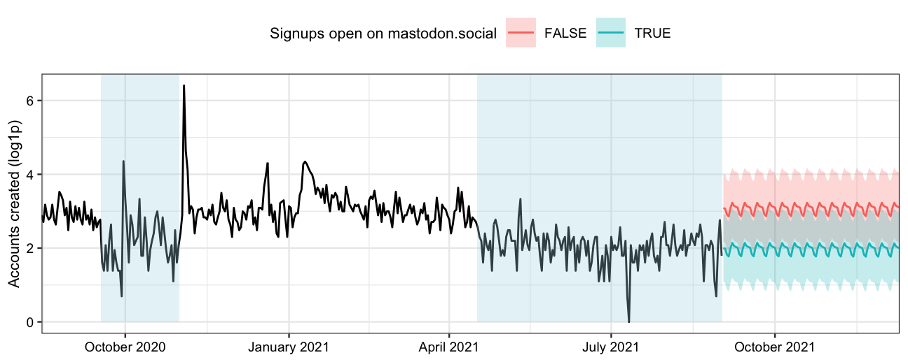
#| label: fig-mastodon-online-forecast
#| fig-cap: "Historical signup counts for mastodon.online and two alternative forecasts based on whether or not mastoodn.social is accepting signups."
#| fig-height: 2.7
#| fig-width:  6.75
#| exec: false
#| fig-env: figure*
model_data <- early.day_counts %>%
  mutate(count = log1p(count)) %>%
  ungroup %>%
  arrange(created_day) %>%
  mutate(day = row_number())

fit <- model_data %>%
  model(arima = ARIMA(count ~ open + day + open:day + fourier(period=7, K=2) + pdq(2,0,0) + PDQ(0,0,0,period=7)))

f_server <- "mastodon.online"

new_data <- tsibble(
  created_day = max(model_data$created_day) + 1:100,
  day = max(model_data$day) + 1:100,
  server = f_server #""
)

Using `created_day` as index variable.

#| label: fig-mastodon-online-forecast
#| fig-cap: "Historical signup counts for mastodon.online and two alternative forecasts based on whether or not mastoodn.social is accepting signups."
#| fig-height: 2.7
#| fig-width:  6.75
#| exec: false
#| fig-env: figure*
model.obj <- fit %>%
  filter(server == f_server) %>%
  select(arima) %>% pull %>% first 

forecast.open <- model.obj %>%
  forecast(new_data=(new_data %>% add_column(open = TRUE))) %>%
  hilo %>% unpack_hilo(`95%`)

forecast.closed <- model.obj %>%
  forecast(new_data=(new_data %>% add_column(open = FALSE))) %>%
  hilo %>% unpack_hilo(`95%`)

hist_data <- as_tibble(model_data) %>% filter(server == f_server) %>% select(created_day, server, count, open) %>% rename(count_mean=count)

bind_rows(
  as_tibble(forecast.open),
  as_tibble(forecast.closed)
) %>%
  rename(count_mean=.mean) %>%
  ggplot(aes(x=created_day, y=count_mean)) +
  geom_line(aes(color=open, group=open)) + #, linetype="dashed") +
  geom_ribbon(aes(ymin=`95%_lower`, ymax=`95%_upper`, group=open, fill=open), alpha=0.25) +
  geom_line(aes(x=created_day, y=count_mean), data=hist_data) + # , color=open, group=open
  geom_rect(data = (hist_data %>% filter(open)),
            aes(xmin = created_day - 0.5, xmax = created_day + 0.5, ymin = 0, ymax = Inf),
            fill = "lightblue", alpha = 0.3) +  # Adjust color and transparency as needed
  labs(
    x = "Date",
    y = "Accounts created (log1p)",
    color = "Signups open on mastodon.social",
    fill = "Signups open on mastodon.social"
  ) +
  scale_x_date(expand = c(0, 0), date_labels = "%B %Y") +
  theme_bw_small_labels() +
  theme(legend.position="top", axis.title.x=element_blank())

Historical signup counts for mastodon.online and two alternative forecasts based on whether or not mastoodn.social is accepting signups.

Relationship between the flagship server and others over time

Relationship between the flagship server and others over time

Competition Among Servers in Attracting Newcomers

Appendix

Push and Pull Model